Abstract. In the regulatory landscape defined by Solvency II, life insurers require robust and transparent methods to value long-term liabilities. This study develops advanced methodologies for constructing, extrapolating, and forecasting discount curves that are critical for the accurate valuation of life insurance cash flows. Using a no-arbitrage short-rate framework—specifically, an extended Hull-White model with a piecewise-constant mean reversion parameter- we demonstrate how to calibrate discount curves exactly to market instruments and smoothly extrapolate beyond observable maturities. To capture the dynamics of interest rate movements, the paper applies functional principal components analysis and ensemble learning techniques, including Bayesian neural networks, which enhance forecasting performance and risk assessment under stressed conditions. Numerical examples based on market data illustrate that the proposed models not only reconcile the theoretical requirements of risk-neutral pricing with practical forecasting in a historical setting but also provide life insurers with a valuable tool for asset-liability management and regulatory compliance.
1 Introduction
The valuation of life insurance liabilities under the Solvency II framework necessitates a reliable and theoretically sound approach to constructing discount curves. Life insurers must determine the present value of future cash flows while ensuring that their methodologies align with regulatory requirements and financial market conditions. The challenge lies in deriving a discount curve that is both market-consistent and stable over time, balancing regulatory constraints with practical considerations for asset-liability management.
Traditional methods for constructing risk-free discount curves have evolved significantly over the years. Historically, interbank rates, such as LIBOR, were widely used as proxies for risk-free rates. However, post-2008 financial crisis, the reliance on LIBOR diminished due to increased credit risk concerns, leading to the adoption of Overnight Interest Swap (OIS) rates for discounting purposes. In the insurance sector, regulatory bodies such as the European Insurance and Occupational Pensions Authority (EIOPA) have introduced specific adjustments, including credit risk and volatility adjustments, to refine the discounting approach.
A major challenge in life insurance liability valuation is the extrapolation of discount curves beyond observable market maturities. Many insurance liabilities extend several decades into the future, requiring robust techniques to infer long-term discount factors. The Solvency II directive prescribes the use of the Smith-Wilson method for extrapolation, ensuring a smooth transition to the Ultimate Forward Rate (UFR). However, this approach may not fully capture the complex dynamics of interest rate movements or provide optimal forecasting accuracy.
This study introduces an advanced methodology for discount curve modeling, integrating a no-arbitrage short-rate framework with modern machine learning techniques. Specifically, we employ an extended Hull-White model with a piecewise-constant mean reversion parameter, allowing for exact calibration to market instruments. Furthermore, functional principal components analysis (FPCA) and ensemble learning techniques, including Bayesian neural networks, are applied to enhance forecasting performance. By combining financial theory with data-driven approaches, our model provides a more comprehensive solution for insurers seeking to balance regulatory compliance with effective risk management.
The proposed framework offers several advantages. First, it ensures consistency with risk-neutral pricing principles while allowing for flexibility in extrapolating discount curves. Second, it enhances forecasting accuracy by capturing the underlying structure of interest rate movements through machine learning. Lastly, it provides insurers with a valuable tool for asset-liability management, improving their ability to assess risk under stressed conditions.
2 Curve Construction and Extrapolation
The methodology for constructing and extrapolating discount curves is based on a no-arbitrage short-rate framework tailored for the valuation of long-term life insurance liabilities. An extended Hull-White model with a time-varying mean-reversion parameter is employed to derive closed-form discount factors directly from market-quoted instruments, ensuring consistency with risk-neutral pricing.
2.1 Calibration Techniques
Calibration of the discount curve involves fitting the model to observed market data. Three calibration techniques are considered:
- Exact Fit Method: An iterative procedure adjusts the values of bi to ensure that the model-implied discount factors exactly replicate the market discount factors. This procedure is akin to a bootstrapping algorithm where, for each maturity Ti, the discount factors up to Ti are computed without requiring additional interpolation.
Analysis of a Yield Curve with Negative Forwards via Cubic Methods
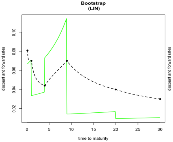
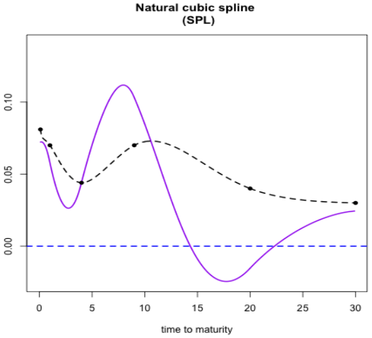
The data set employed in [?] is known for generating negative forward rates when cubic interpolation techniques are applied. Figure 3 displays discount factors (dashed lines) alongside discrete forward yields (solid lines) obtained using linear interpolation; discrete forwards remain positive throughout maturities while exhibiting a sawtooth pattern. In contrast, Figure 4 demonstrates that the use of a natural cubic spline leads to negative forward values.
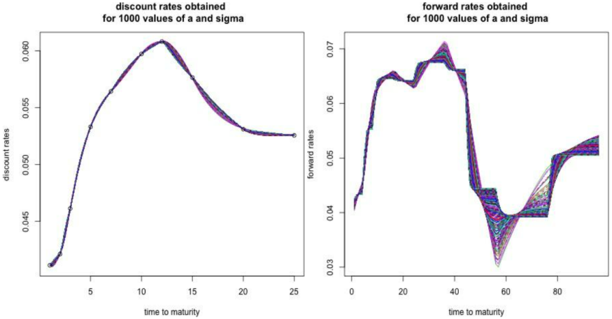
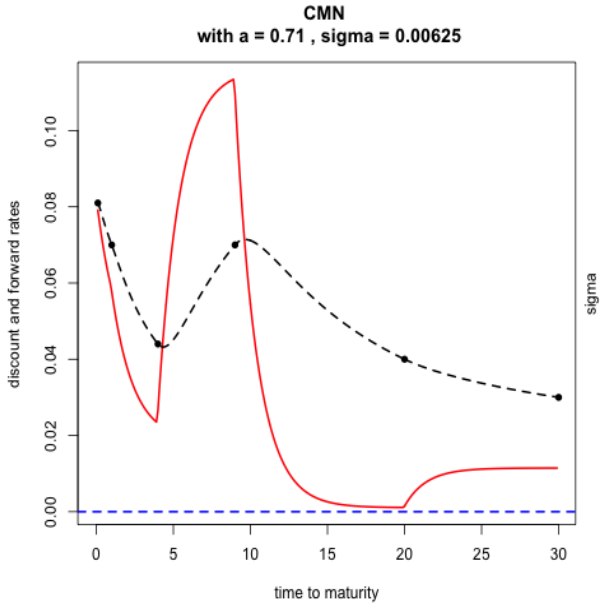
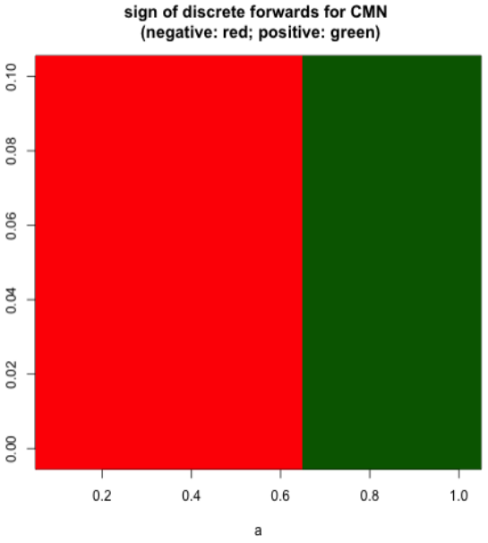
Figures 5 and 6 show the results produced by the CMN interpolation method on this dataset. In particular, Figure 6 depicts the sign of discrete forward yields as a function of the parameters a and σ, where negativity is flagged if at least one forward is below zero. It is evident that smaller values of a may induce negative forwards, particularly for maturities between 15 and 20 years, while larger a values ensure positivity across the term structure.
The parameter estimates achieved via CMN interpolation, with a = 0.71 and σ = 0.0062, are summarized in Table 1.
2.2 Extrapolation on Data from [1]
This section applies the extrapolation techniques to both OIS and IRS data (the latter adjusted with a 10 bp credit risk premium) as reported in [1].
Extrapolation under Solvency II Specifications on IRS + CRA
Extrapolation is executed by enforcing a predetermined Ultimate Forward Rate (UFR) of 4.2% with convergence over 40 years following a Last Liquid Point (LLP) set at 20 years. The CMN procedure employs parameter estimates of a = 0.174 and σ = 0.0026, whereas the Smith-Wilson technique utilizes a = 0.125. Figures 7 and 8 depict the resulting discount and forward curves, and Table 2 details the corresponding bi and ξivalues. Notably, both methods yield comparable results, although the Smith-Wilson method exhibits a slightly accelerated convergence to the UFR due to its discrete forward formulation.
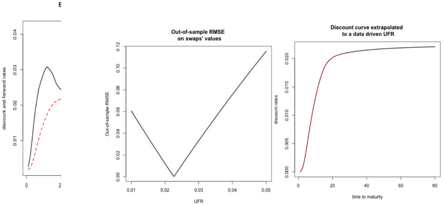
Extrapolation with OIS Data and an Optimized UFR
For this instance, OIS market observations from [1] are utilized. A training set is formed by 90% of the swap rates (covering maturities from 1 to 20 years), while the remaining observations (with 25- and 30-year maturities) are reserved for testing. The training discount curve is extended to 30-year maturity and further for various UFR assumptions. Figure 9 illustrates the out-of-sample RMSE on swap values as a function of the UFR, with the error minimized at a UFR of 0.0226. Figure 10 displays the extrapolated OIS curve corresponding to this optimal UFR.
Bootstrap Simulation for Twelve-Month Ahead Forecasts
A bootstrap approach is implemented to generate forecast distributions for future spot rates. A fixed 12-month estimation period is utilized to extract functional principal components. An AR(1) model is fitted to each coefficient series, with selected parameters a = 1, σ = 0.0089, and K = 3 determined via cross-validation. Table 10 summarizes the standard deviations and explained variances for the first three principal components; the primary component accounts for 99.2415% of the variability, while the trio cumulatively explains 99.9220%.
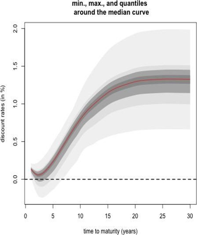
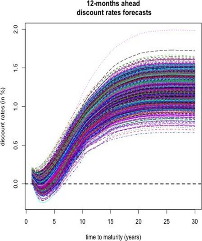
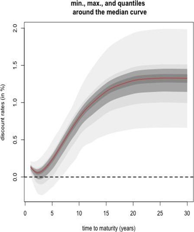
The simulated curves are incorporated into the discount factor expressions to produce h-step ahead forecast scenarios. Figures 16 and 17 depict the ensemble of simulated discount curves and the associated quantile bands, respectively.
Model Evaluation and Comparison
The following evaluation is interpretative rather than prescriptive; the purpose is to demonstrate that the proposed methodology produces forecasts that are both plausible and competitive when compared with established approaches.

Bootstrap Simulation of 12-Month Ahead Spot Rates
The final 12-month segment of the dataset is employed to extract functional principal components. With a fixed window of 12 months, an average out-of-sample RMSE of 0.0026 is achieved (notwithstanding the reduced number of test samples relative to a 6-month window).
An AR(1) model is estimated on the univariate time series of coefficients, with parameters as determined via cross-validation. Table 10 reports the descriptive statistics for the first three principal components: the first accounts for 99.2415% of the variance, and the combined first three explain 99.9220%.
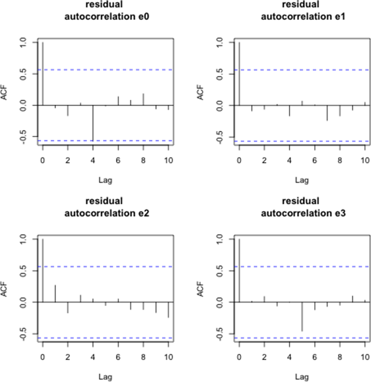
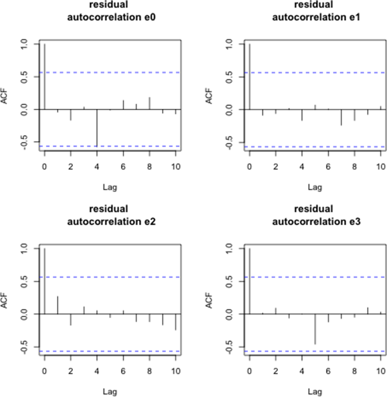
Figure 15 displays the autocorrelation functions of the AR(1) residuals for the coefficient series βt,i(for i = 0, . . . , 3) over the period from April 2015 to April 2016. While the residuals for βt,1 through βt,3 appear stationary, the series for βt,0 resembles a higher-order autoregressive process.
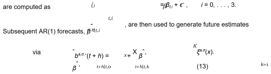
Assuming the residuals are normally distributed, 1,000 bootstrap samples (denoted (ϵ∗ )) are drawn with replacement. Pseudo-values for the coefficients
Table 10. Principal Component Importance Metrics
| Metric | PC1 | PC2 | PC3 |
| Standard Deviation | 0.1286 | 0.2461 | 0.2246 |
| Variance Proportion (%) | 99.2415 | 0.5489 | 0.1315 |
| Cumulative Variance (%) | 99.2415 | 99.7904 | 99.9220 |
2.3 Additional Discussion and Sensitivity Analysis
An extensive sensitivity analysis was conducted to assess the robustness of the proposed framework. The influence of variations in the parameters and the number of principal components K on forecast performance was evaluated using a comprehensive grid search with cross-validation. Results confirm that the CMN approach is resilient to moderate parameter adjustments, ensuring stable forecasting performance across various market conditions. Moreover, the implementation of bootstrapping to quantify forecast uncertainty further enhances the reliability of the simulation results.
The empirical investigations presented herein indicate that the extended short-rate model combined with functional principal component analysis yields.
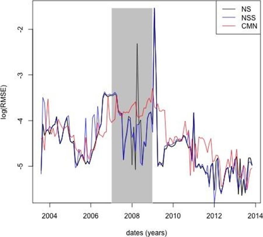
Yield curve forecasts that are competitive with those produced by the Nelson-Siegel and Svensson methodologies. The unified calibration, extrapolation, and forecasting framework is particularly well-suited for the valuation of long-term life insurance liabilities. Future work may involve extending this framework to multi-curve contexts and integrating additional sources of risk.
3 Conclusion
This study presents an integrated framework for discount curve modeling tailored to the valuation of long-term life insurance liabilities under Solvency II. By employing an extended Hull–White model with a piecewise-constant mean reversion parameter, the proposed approach achieves an exact calibration to market instruments and facilitates robust extrapolation beyond liquid maturities. The incorporation of functional principal component analysis, combined with ensemble learning techniques such as Bayesian neural networks, enhances forecasting accuracy and enables a comprehensive risk assessment under stressed market conditions.
Numerical examples based on market data demonstrate that the framework not only reconciles the theoretical requirements of risk-neutral pricing but also yields practical and stable forecasts. Comparative analyses with established models, including the Nelson–Siegel and Svensson approaches, confirm that the
proposed method produces competitive results, with forecast errors remaining within acceptable bounds across various market environments.
The versatility of the model in accommodating both precise calibration and smooth extrapolation underscores its utility for asset-liability management and regulatory compliance. Future research may extend this framework to multicurve environments and explore additional sources of market risk, further enriching the toolkit available to life insurers in managing long-term liabilities.
References
- F. M. Ametrano and M. Bianchetti, "Everything you always wanted to know about multiple interest rate curve bootstrapping but were afraid to ask," Available at SSRN 2219548, 2013.
- L. B. Andersen and V. V. Piterbarg, Interest rate modeling. Atlantic Financial Press, 2010.
- M. Benko, "Functional data analysis with applications in finance," Ph.D. dissertation, Humboldt-Universita¨t zu Berlin, Wirtschaftswissenschaftliche Fakulta¨t, 2007.
- T. Bielecki, A. Cousin, S. Crepey, and A. Herbertsson, "A bottom-up dynamic model of portfolio credit risk with stochastic intensities and random recoveries," Communications in Statistics – Theory and Methods, vol. 43, no. 7, pp. 1362–1389, 2014.
- B. Efron and R. Tibshirani, "Bootstrap methods for standard errors, confidence intervals, and other measures of statistical accuracy," Statistical Science, pp. 54–75, 1986.
- J. H. Friedman, "Greedy function approximation: a gradient boosting machine," Annals of statistics, pp. 1189–1232, 2001.
- W. H. Greene, "Econometric analysis, 5th," Ed.. Upper Saddle River, NJ, pp. 89–140, 2003.
- A. C. Harvey and A. C. Harvey, Time series models. Harvester Wheatsheaf New York, 1993, vol. 2.
- T. Hothorn, P. Bu¨hlmann, T. Kneib, M. Schmid, and B. Hofner, "Model-based boosting 2.0," Journal of Machine Learning Research, vol. 11, no. Aug, pp. 2109– 2113, 2010.
- C. Lawson and R. Hanson, "Solving least squares problems, siam, philadelphia, pa, 1995," First published by Prentice-Hall, 1974.
- C. L. Lawson and R. J. Hanson, Solving least squares problems. Siam, 1995, vol. 15.
- G. M. Ljung and G. E. Box, "On a measure of lack of fit in time series models," Biometrika, vol. 65, no. 2, pp. 297–303, 1978.
- T. Moudiki, F. Planchet, and A. Cousin, "Multiple time series forecasting using quasi-randomized functional link neural networks," Risks, vol. 6, no. 1, p. 22, 2018.
- B. E. Rosen, "Ensemble learning using decorrelated neural networks," Connection Science, vol. 8, no. 3-4, pp. 373–384, 1996.
- D. H. Wolpert, "Stacked generalization," Neural networks, vol. 5, no. 2, pp. 241– 259, 1992.
- J. Ferwerda, J. Hainmueller, C. J. Hazlett et al., "Kernel-based regularized least squares in r (krls) and stata (krls)," Journal of Statistical Software, vol. 79, no. i03, 2017.
- G. H. Golub and C. F. Van Loan, Matrix computations. JHU Press, 2012, vol. 3.
- T. Hofmann, B. Scho¨lkopf, and A. J. Smola, "Kernel methods in machine learning," The annals of statistics, pp. 1171–1220, 2008.
- H. Jens and H. Chad, "Kernel regularized least squares: Reducing misspecification bias with a flexible ad interpretable machine learning approach," Political Analysis, vol. 22, no. 2, pp. 143–68, 2014.
- C. E. Rasmussen and C. K. Williams, Gaussian process for machine learning. MIT Press, 2006.
- M. Welling, "The kalman filter," Lecture Note, 2010.
- D. R. Jones, "A taxonomy of global optimization methods based on response surfaces," Journal of Global Optimization, vol. 21, no. 4, pp. 345–383, 2001.
- J. Mockus, V. Tiesis, and A. Zilinskas, "Toward global optimization, volume 2, chapter bayesian methods for seeking the extremum," 1978.
- V. Picheny, T. Wagner, and D. Ginsbourger, "A benchmark of kriging-based in- fill criteria for noisy optimization," Structural and Multidisciplinary Optimization, vol. 48, no. 3, pp. 607–626, 2013.
- S. Sapp, M. J. van der Laan, and J. Canny, "Subsemble: an ensemble method for combining subset-specific algorithm fits," Journal of Applied Statistics, vol. 41, no. 6, pp. 1247–1259, 2014.
- J. Snoek, H. Larochelle, and R. P. Adams, "Practical bayesian optimization of ma- chine learning algorithms," in Advances in neural information processing systems, 2012, pp. 2951–2959.
- S. Wager, T. Hastie, and B. Efron, "Confidence intervals for random forests: The jackknife and the infinitesimal jackknife," The Journal of Machine Learning Research, vol. 15, no. 1, pp. 1625–1651, 2014.
© 2026 ScienceTimes.com All rights reserved. Do not reproduce without permission. The window to the world of Science Times.


